Quick Guide from AS to AP Mechanics
Unit 1: Kinematics
v m i d x = v 0 2 + v t 2 2 v_{mid\ x} = \sqrt{\dfrac{v_0^2 + v_t^2}2} v mi d x = 2 v 0 2 + v t 2
Unit 2: Force & Translational Dynamics
Resistive Force
Turbulent Drag :
D = 1 2 C ρ A v 2 D = \dfrac{1}{2} C \rho A v^2 D = 2 1 C ρ A v 2
C C C ρ \rho ρ A A A v v v
Terminal velocity of free fall: v max = 2 F g C ρ A v_{\max} = \sqrt{\dfrac{2F_g}{C \rho A}} v m a x = C ρ A 2 F g
θ = ϕ + ω t \theta = \phi + \omega t θ = ϕ + ω t
s ⃗ = ( r cos ( ϕ + ω t ) , r sin ( ϕ + ω t ) ) \vec{s} = (r \cos(\phi + \omega t), r \sin(\phi + \omega t)) s = ( r cos ( ϕ + ω t ) , r sin ( ϕ + ω t ))
v ⃗ = d s ⃗ d t = ( − r ω sin ( ϕ + ω t ) , r ω cos ( ϕ + ω t ) ) \vec{v} = \dfrac{d\vec{s}}{dt} = (-r \omega \sin(\phi + \omega t), r \omega \cos(\phi + \omega t)) v = d t d s = ( − r ω sin ( ϕ + ω t ) , r ω cos ( ϕ + ω t ))
a ⃗ = d v ⃗ d t = ( − r ω 2 cos ( ϕ + ω t ) , − r ω 2 sin ( ϕ + ω t ) ) = − ω 2 s ⃗ \vec{a} = \dfrac{d\vec{v}}{dt} = (-r \omega^2 \cos(\phi + \omega t), -r\omega^2 \sin(\phi + \omega t)) = - \omega^2 \vec{s} a = d t d v = ( − r ω 2 cos ( ϕ + ω t ) , − r ω 2 sin ( ϕ + ω t )) = − ω 2 s
Therefore, s ⃗ \vec{s} s a ⃗ \vec{a} a s ⃗ \vec{s} s a ⃗ \vec{a} a
a = ω 2 r = v 2 r a = \omega^2 r = \dfrac{v^2}r a = ω 2 r = r v 2
General Circular Motion
s ⃗ = ( r cos θ , r sin θ ) \vec{s} = (r\cos\theta, r\sin\theta) s = ( r cos θ , r sin θ )
v ⃗ = ( − r ω sin θ , r ω cos θ ) \vec{v} = (-r \omega \sin\theta, r \omega \cos\theta) v = ( − r ω sin θ , r ω cos θ ) ω = d θ d t \omega = \dfrac{d\theta}{dt} ω = d t d θ
Gravitation Force
F ⃗ = − G m 1 m 2 r 2 ⋅ r ^ \vec{F} = - G \dfrac{m_1m_2}{r^2} \cdot \hat{r} F = − G r 2 m 1 m 2 ⋅ r ^ r ^ \hat{r} r ^
Gravitation Inside
For a shell, its gravitational force to an object inside it is 0. Therefore, we only need to calculate the sub sphere inside the object to find out the gravitation.
Position of Center of Mass
For a line with n discrete particles, x c o m = 1 M ∑ i = 1 n m i x i x_{com} = \dfrac1M \sum\limits_{i=1}^n m_i x_i x co m = M 1 i = 1 ∑ n m i x i y c o m y_{com} y co m z c o m z_{com} z co m
The position of the center of mass is fixed when the object is at equilibrium.
The velocity of the center of mass tells the velocity of a specific point. Since the net external force is zero, the velocity of that specific point cannot change. Therefore, the center of mass is fixed.
Notice that the center of mass does not change relative to the inertial frame of reference but not the relative position to the object itself. This is because we measure the velocity relative to the frame of reference but not a point on the object. The center of mass can change its relative position on the object if the object moves, but not relative to the frame of reference.
To understand this point, check AP Mechanics Problem Collection#1 .
Unit 3: Work, Energy, and Power
Potential Energy
Δ U = − W = − ∫ F ⃗ ⋅ d r ⃗ \Delta U = - W = - \int \vec{F} \cdot d\vec{r} Δ U = − W = − ∫ F ⋅ d r
⟹ U ( r ) − U ( ∞ ) = U ( r ) = − ∫ ∞ r F ⃗ ⋅ d r ⃗ \implies U(r) - U(\infty) = U(r) = - \int_\infty^r \vec{F} \cdot d \vec{r} ⟹ U ( r ) − U ( ∞ ) = U ( r ) = − ∫ ∞ r F ⋅ d r
Conservative Force
A force that does zero net work over a closed path. It is path-independent and can be described by a potential energy function.
Because the path does not matter to the work done by a conservative force, we can determine the force at each point as F ( x ) = − d U ( x ) d x F(x) = - \dfrac{dU(x)}{dx} F ( x ) = − d x d U ( x ) U ( x ) U(x) U ( x )
Conservation of Mechanical Energy
In a system, if only conservative forces are doing work, the mechanical energy of the system conserves.
Unit 4: Linear Momentum
Law of Motion for the Center of Mass
v c o m = 1 M ∑ i = 1 N m i v i v_{com} = \dfrac1M \sum\limits_{i=1}^N m_iv_i v co m = M 1 i = 1 ∑ N m i v i
a c o m = 1 M ∑ i = 1 N m i a i a_{com} = \dfrac1M \sum\limits_{i=1}^N m_ia_i a co m = M 1 i = 1 ∑ N m i a i
Linear Momentum
Without external forces, the linear momentum is conserved.
Impulse
The change in an object's momentum caused by a net external force acting over a specific time interval
J = ∫ t i t f F n e t ( t ) d t = Δ P J = \int_{t_i}^{t_f} F_{net}(t) dt = \Delta P J = ∫ t i t f F n e t ( t ) d t = Δ P
Elastic & Inelastic Collision
Besides elasticity, a collision can also be categorized as a frontal or a oblique collision.
If a collision is perfectly inelastic, two objects will have the same terminal velocity.
If a collision is perfectly elastic and frontal, the absolute value of the velocity difference is the same before and after the collision. When the masses of two are equal as well, two objects will swap velocity.
Systems with Varying Mass
To analyze a flying rocket:
M v = d M ( v − v r e l ) + ( M − d m ) ( v + d v ) Mv = dM (v-v_{rel}) + (M-dm)(v+dv) M v = d M ( v − v r e l ) + ( M − d m ) ( v + d v ) v r e l v_{rel} v r e l d M dM d M
− d M ⋅ v r e l = M ⋅ d v -dM \cdot v_{rel} = M \cdot dv − d M ⋅ v r e l = M ⋅ d v
To calculate thrust R R R
− d M d t ⋅ v r e l = M ⋅ d v d t = M a = R - \dfrac{dM}{dt} \cdot v_{rel} = M \cdot \dfrac{dv}{dt} = Ma = R − d t d M ⋅ v r e l = M ⋅ d t d v = M a = R
⟹ R = − d M d t v r e l \implies R = - \dfrac{dM}{dt} v_{rel} ⟹ R = − d t d M v r e l
To calculate the change in the velocity of the rocket Δ v \Delta v Δ v
d v = − v r e l ⋅ 1 M d M dv = - v_{rel} \cdot \dfrac{1}{M} dM d v = − v r e l ⋅ M 1 d M
⟹ Δ v = ∫ v 0 v d v = − v r e l ⋅ ∫ M 0 M 1 M d M \implies \Delta v = \int_{v_0}^{v} dv = - v_{rel} \cdot \int_{M_0}^{M} \dfrac{1}{M} dM ⟹ Δ v = ∫ v 0 v d v = − v r e l ⋅ ∫ M 0 M M 1 d M
⟹ Δ v = − v r e l ⋅ ln ( M M 0 ) = v r e l ⋅ ln ( M 0 M ) \implies \Delta v = - v_{rel} \cdot \ln(\dfrac{M}{M_0}) = v_{rel} \cdot \ln(\dfrac{M_0}{M}) ⟹ Δ v = − v r e l ⋅ ln ( M 0 M ) = v r e l ⋅ ln ( M M 0 )
We can see that the more Δ M \Delta M Δ M Δ v \Delta v Δ v
Unit 5: Torque & Rotational Dynamics
Angular Position
Angular position θ \theta θ θ = s r \theta = \dfrac{s}{r} θ = r s s s s r r r
A counterclockwise angular displacement is positive.
Angular Velocity & Acceleration
Angular velocity ω = Δ θ Δ t \omega = \dfrac{\Delta \theta}{\Delta t} ω = Δ t Δ θ s − 1 s^{-1} s − 1
v = ω r v = \omega r v = ω r
Angular acceleration α = Δ ω Δ t \alpha = \dfrac{\Delta \omega}{\Delta t} α = Δ t Δ ω s − 2 s^{-2} s − 2
a = α r a = \alpha r a = α r
Rotation Kinematics
The equations are the same to linear kinematics:
ω = ω 0 + α t \omega = \omega_0 + \alpha t ω = ω 0 + α t θ = ω 0 t + 1 2 α t 2 \theta = \omega_0t + \dfrac12 \alpha t^2 θ = ω 0 t + 2 1 α t 2 θ = ω t − 1 2 α t 2 \theta = \omega t - \dfrac12 \alpha t^2 θ = ω t − 2 1 α t 2 2 α θ = ω 2 − ω 0 2 2\alpha \theta = \omega^2 - \omega_0^2 2 α θ = ω 2 − ω 0 2 ω = ( ω 0 + ω ) t 2 \omega = \dfrac{(\omega_0 + \omega) t}2 ω = 2 ( ω 0 + ω ) t
Kinetic Energy of Rotation
K = ∑ 1 2 m v 2 = ∑ 1 2 m ( ω r ) 2 K = \sum \dfrac12 mv^2 = \sum \dfrac12 m(\omega r)^2 K = ∑ 2 1 m v 2 = ∑ 2 1 m ( ω r ) 2
Notice that ∑ m r 2 \sum mr^2 ∑ m r 2 I = ∑ m r 2 = ∫ r 2 d m I = \sum mr^2 = \int r^2 dm I = ∑ m r 2 = ∫ r 2 d m I I I
K = 1 2 I ω 2 K = \dfrac12 I \omega^2 K = 2 1 I ω 2
Moment of Inertia
I = ∑ m r 2 = ∫ r 2 d m I = \sum mr^2 = \int r^2 dm I = ∑ m r 2 = ∫ r 2 d m
To infer the formula of the moment of inertia of an object, we need to transform d m dm d m d e n s i t y ( θ ) ⋅ d l density(\theta) \cdot dl d e n s i t y ( θ ) ⋅ d l
Take a point on the ring with mass d m dm d m d m = λ d l dm = \lambda dl d m = λ d l λ \lambda λ d l dl d l Δ I = r 2 λ d l \Delta I = r^2 \lambda dl Δ I = r 2 λ d l I = ∫ Δ I = ∫ 0 2 π r r 2 λ d l = r 2 m I = \int \Delta I = \int_0^{2\pi r} r^2 \lambda dl = r^2 m I = ∫ Δ I = ∫ 0 2 π r r 2 λ d l = r 2 m ∫ 0 2 π r λ d l = m \int_0^{2\pi r} \lambda dl = m ∫ 0 2 π r λ d l = m
To quickly compare the moment of inertia for objects with the same mass but different shapes, we can apply the Mass Concentration Rule :
The farther the mass is pushed away from the axis of rotation, the larger its moment of inertia is.
Parallel Axis Theorem
The moment of inertia of an object rotating at an axis deviating to its center of mass can be calculated as I = I c o m + m d 2 I = I_{com} + md^2 I = I co m + m d 2 d d d
Torque
Torque τ = F r ⋅ r = F ⃗ × r ⃗ \tau = F_r \cdot r = \vec{F} \times \vec{r} τ = F r ⋅ r = F × r F r F_r F r
τ = F r ⋅ r = m a ⋅ r = m α r ⋅ r = m r 2 ⋅ α = I α \tau = F_r \cdot r = ma \cdot r = m \alpha r \cdot r = mr^2 \cdot \alpha = I\alpha τ = F r ⋅ r = ma ⋅ r = m α r ⋅ r = m r 2 ⋅ α = I α
Unit 6: Energy & Momentum of Rotating Systems
Kinetic Energy of An Rigid System
K = K t r a n s + K r o t = 1 2 m v 2 + 1 2 I ω 2 K = K_{trans} + K_{rot} = \dfrac12 mv^2 + \dfrac12 I \omega^2 K = K t r an s + K r o t = 2 1 m v 2 + 2 1 I ω 2
Only when rolling without slipping, v = ω r v = \omega r v = ω r a = α r a = \alpha r a = α r
Rotation Work
W = 1 2 I ( ω 2 − ω 0 2 ) = τ ⋅ d θ W = \dfrac12 I (\omega^2 - \omega_0^2) = \tau \cdot d\theta W = 2 1 I ( ω 2 − ω 0 2 ) = τ ⋅ d θ
P = d W d t = τ ω P = \dfrac{dW}{dt} = \tau \omega P = d t d W = τ ω
Angular Momentum & Impulse
Angular momentum L ⃗ = r ⃗ × p ⃗ = m r ⃗ × v ⃗ \vec{L} = \vec{r} \times \vec{p} = m \vec{r} \times \vec{v} L = r × p = m r × v L = m r v sin θ L = mrv\sin\theta L = m r v sin θ p ⃗ \vec{p} p r ⃗ \vec{r} r
τ ⃗ = L ⃗ d t \vec{\tau} = \dfrac{\vec{L}}{dt} τ = d t L
Total momentum L ⃗ t o t = ∑ r ⃗ × v ⃗ \vec{L}_{tot} = \sum \vec{r} \times \vec{v} L t o t = ∑ r × v
⟹ d L ⃗ t o t d t = ∑ r ⃗ × F ⃗ n e t = τ ⃗ n e t , e x t \implies \dfrac{d\vec{L}_{tot}}{dt} = \sum \vec{r} \times \vec{F}_{net} = \vec{\tau}_{net, ext} ⟹ d t d L t o t = ∑ r × F n e t = τ n e t , e x t
Therefore, if the net external torque of a system is zero, the total angular momentum is preserved.
The conservation of angular momentum and linear momentum is independent. There is no such conservation of (L L L p p p
For a system rotating at a fixed axis, we only need to consider the angular momentum around the axis. Therefore:
L = ∑ m r p e r v = ∑ m r p e r 2 ω = I ω L = \sum mr_{per}v = \sum mr^2_{per}\omega = I \omega L = ∑ m r p er v = ∑ m r p er 2 ω = I ω r p e r r_{per} r p er
Angular impulse Δ L = ∫ t 1 t 2 τ n e t d t \Delta L = \int_{t_1}^{t_2} \tau_{net} dt Δ L = ∫ t 1 t 2 τ n e t d t
Motion of Orbiting Satellites
v = G M r v = \sqrt{\dfrac{GM}{r}} v = r GM
ω = G M r 3 \omega = \sqrt{\dfrac{GM}{r^3}} ω = r 3 GM
T 2 M G = 4 π 2 r 3 T^2 MG = 4 \pi^2 r^3 T 2 M G = 4 π 2 r 3
Potential Energy of Orbiting Satellites
F ⃗ ⋅ d r ⃗ = − G M m r 2 d r \vec{F}\cdot d\vec{r} = - G \dfrac{Mm}{r^2} dr F ⋅ d r = − G r 2 M m d r
⟹ U ( r ) = − ∫ ∞ r ( − G M m r 2 ) d r = G M m ∫ ∞ r 1 r 2 d r = − G M m r \implies U(r) = - \int_\infty^r (-G\dfrac{Mm}{r^2}) dr = GMm \int_\infty^r \dfrac{1}{r^2} dr = - G \dfrac{Mm}r ⟹ U ( r ) = − ∫ ∞ r ( − G r 2 M m ) d r = GM m ∫ ∞ r r 2 1 d r = − G r M m
K = 1 2 m v 2 = G M m 2 r K = \dfrac12 mv^2 = G\dfrac{Mm}{2r} K = 2 1 m v 2 = G 2 r M m
K t o t = − G M m 2 r K_{tot} = -G\dfrac{Mm}{2r} K t o t = − G 2 r M m
Linear-to-Angular Translation
Linear
Angular
Mass m m m
Rotational Inertia I I I
Velocity v v v
Angular Velocity ω \omega ω
Acceleration a a a
Angular Acceleration α \alpha α
Force F F F
Torque τ \tau τ
Kinetic Energy K = 1 2 m v 2 K = \dfrac{1}{2}mv^2 K = 2 1 m v 2
Rotational Kinetic Energy K = 1 2 I ω 2 K = \dfrac{1}{2}I\omega^2 K = 2 1 I ω 2
Work W = Δ K W = \Delta K W = Δ K
Rotational Work W = Δ K W = \Delta K W = Δ K
Momentum p p p
Rotational Momentum L L L
Unit 7: Oscillations
Steps to Solve Simple Harmonic Motion
You may first read the sections below that come back to this. Though the formulas in the sections may appear to be complex and scary, they can be mostly solved in the following step.
Step
Action
Linear Equation
Angular Equation
1
Identify the restoring force/torque
F n e t F_{net} F n e t τ n e t \tau_{net} τ n e t
2
Relate it to displacement
F n e t = − k x F_{net} = -kx F n e t = − k x τ n e t = − κ θ \tau_{net} = - \kappa \theta τ n e t = − κ θ
3
Use Newton's 2nd Law
a = − k m x a = - \dfrac{k}m x a = − m k x α = − κ I θ \alpha = - \dfrac{\kappa}I \theta α = − I κ θ
4
Identify ω 2 \omega^2 ω 2
a = − ω 2 x a = - \omega^2 x a = − ω 2 x α = − ω 2 θ \alpha = -\omega^2 \theta α = − ω 2 θ
5
Extract ω \omega ω
ω = k m \omega = \sqrt{\dfrac k m} ω = m k ω = κ I \omega = \sqrt{\dfrac \kappa I} ω = I κ
6
State the period
T = 2 π ω T = \dfrac{2\pi}\omega T = ω 2 π T = 2 π ω T = \dfrac{2\pi}\omega T = ω 2 π
Dynamics of Horizontal Spring-Block Oscillator
According to Hooke's Law, the restoring force F s = − k x = m a = m d 2 x d t 2 F_s = -kx = ma = m \dfrac{d^2x}{dt^2} F s = − k x = ma = m d t 2 d 2 x
d 2 x d t 2 = − k m x \dfrac{d^2x}{dt^2} = -\dfrac k m x d t 2 d 2 x = − m k x ω = k m \omega = \sqrt{\dfrac k m} ω = m k d 2 x d t 2 = − ω 2 x \dfrac{d^2x}{dt^2} = - \omega^2 x d t 2 d 2 x = − ω 2 x
One solution of the above equation is:
x = A c o s ( ω t ) x = A cos(\omega t) x = A cos ( ω t )
v = d x d t = − A ω sin ( ω t ) v = \dfrac{dx}{dt} = -A\omega\sin(\omega t) v = d t d x = − A ω sin ( ω t ) ω t = π 2 \omega t=\dfrac\pi 2 ω t = 2 π v v v
a = d v d t = − A ω 2 cos ( ω t ) = − ω 2 x a = \dfrac{dv}{dt} = -A\omega^2 \cos(\omega t) = -\omega^2 x a = d t d v = − A ω 2 cos ( ω t ) = − ω 2 x
T = 2 π ω = 2 π m k T = \dfrac{2\pi}{\omega} = 2\pi \sqrt{\dfrac m k} T = ω 2 π = 2 π k m
Energy of Horizontal Spring-Block Oscillator
K = 1 2 m v 2 = 1 2 m ( − A ω sin ( ω t ) ) 2 = 1 2 m A 2 ω 2 sin 2 ( ω t ) K = \dfrac 1 2 mv^2 = \dfrac 1 2 m (-A \omega \sin(\omega t))^2 = \dfrac 1 2 m A^2 \omega^2 \sin^2(\omega t) K = 2 1 m v 2 = 2 1 m ( − A ω sin ( ω t ) ) 2 = 2 1 m A 2 ω 2 sin 2 ( ω t )
When U = 0 U = 0 U = 0 K K K 1 2 m A 2 ω 2 \dfrac 1 2 mA^2 \omega^2 2 1 m A 2 ω 2
U = 1 2 k x 2 = 1 2 k ( A cos ( ω t ) ) 2 = 1 2 k A 2 cos 2 ( ω t ) U = \dfrac 1 2 kx^2 = \dfrac 1 2 k (A \cos(\omega t))^2 = \dfrac 1 2 kA^2 \cos^2(\omega t) U = 2 1 k x 2 = 2 1 k ( A cos ( ω t ) ) 2 = 2 1 k A 2 cos 2 ( ω t )
When K = 0 K = 0 K = 0 U U U 1 2 k A 2 \dfrac 1 2 k A^2 2 1 k A 2
Total energy E = K + U = 1 2 m A 2 ω 2 sin 2 ( ω t ) + 1 2 k A 2 cos 2 ( ω t ) E = K + U = \dfrac 1 2 m A^2 \omega^2 \sin^2(\omega t) + \dfrac 1 2 kA^2 \cos^2(\omega t) E = K + U = 2 1 m A 2 ω 2 sin 2 ( ω t ) + 2 1 k A 2 cos 2 ( ω t ) ω 2 = k m \omega^2 = \dfrac k m ω 2 = m k m ω 2 = k m \omega^2 = k m ω 2 = k
E = 1 2 k A 2 ( sin 2 ( ω t ) + cos 2 ( ω t ) ) = 1 2 k A 2 E = \dfrac 1 2 kA^2(\sin^2(\omega t) + \cos^2(\omega t)) = \dfrac 1 2 k A^2 E = 2 1 k A 2 ( sin 2 ( ω t ) + cos 2 ( ω t )) = 2 1 k A 2
Therefore, the energy of the oscillator conserves.
Inclined Spring-Block Oscillator
All equations are the same to horizontal spring-block oscillator.
Torsion Pendulum
d 2 θ d t 2 = − ω 2 θ \dfrac{d^2\theta}{dt^2} = - \omega^2 \theta d t 2 d 2 θ = − ω 2 θ ω = K I \omega = \dfrac K I ω = I K K K K
One solution of the above equation is:
θ = A cos ( ω t ) \theta = A \cos(\omega t) θ = A cos ( ω t )
Ω = d θ d t = − A ω sin ( ω t ) \Omega = \dfrac{d\theta}{dt} = -A\omega\sin(\omega t) Ω = d t d θ = − A ω sin ( ω t )
α = d Ω d t = − ω 2 θ \alpha = \dfrac{d\Omega}{dt} = -\omega^2 \theta α = d t d Ω = − ω 2 θ
T = 2 π I K T = 2\pi \sqrt{\dfrac I K} T = 2 π K I
Simple Pendulum
Because θ \theta θ sin ( θ ) = θ \sin(\theta) = \theta sin ( θ ) = θ
τ = − L m g θ = − K θ \tau = - L mg \theta = -K\theta τ = − L m g θ = − K θ K = L m g K = Lmg K = L m g
T = 2 π L g T = 2\pi \sqrt{\dfrac L g} T = 2 π g L
Physical Pendulum
Because θ \theta θ sin ( θ ) = θ \sin(\theta) = \theta sin ( θ ) = θ
r = − m g sin ( θ ) h = − m g θ h r = -mg \sin(\theta) h = -mg\theta h r = − m g sin ( θ ) h = − m g θ h
α = − m g h I θ = − ω θ \alpha = - \dfrac{mgh}{I} \theta = - \omega \theta α = − I m g h θ = − ω θ ω = m g h I \omega = \sqrt{\dfrac{mgh}{I}} ω = I m g h
T = 2 π I m g h T = 2\pi \sqrt{\dfrac I {mgh}} T = 2 π m g h I
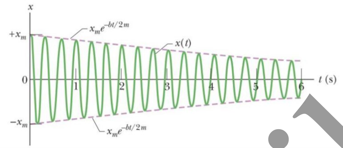
Damped Simple Harmonic Motion
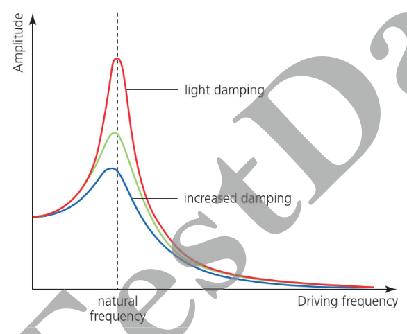
Forced Oscillations & Resonance